Overview
Census data are invaluable to social science research and are available through the census API. Unfortunately, adding census data into a study is time-consuming. This is because census tables are complex, geographic units are confusing, the American Community Survey sampling framework is nuanced, and data harmonization over time requires significant expertise.
To address this problem, we are developing tools to make appending census data to NCCS data series easier. Our aim is a seamlessly integrated and intuitive process requiring minimal effort from users.
GEOGRAPHIC CROSSWALK FILES
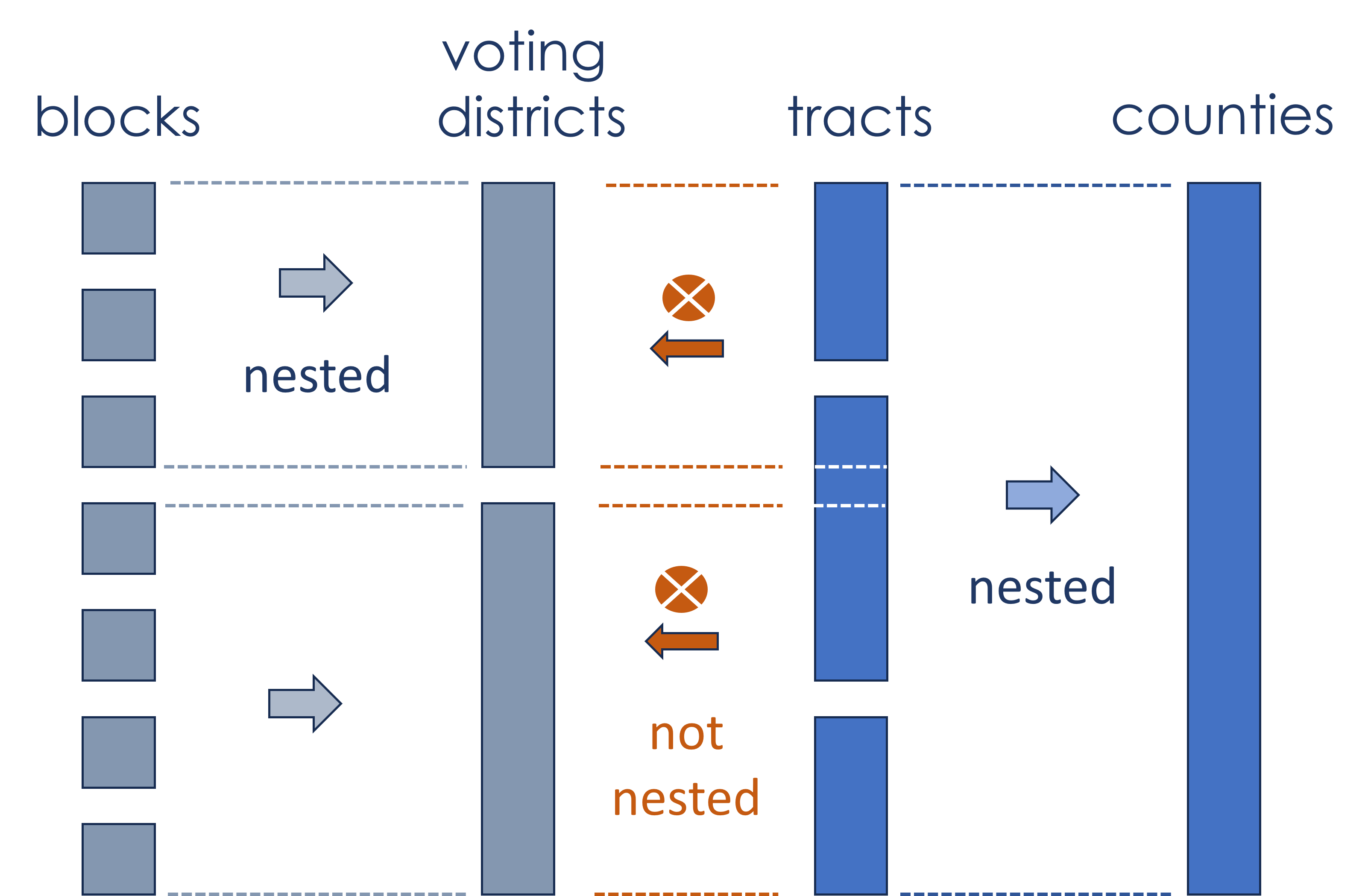
Any census-designated geography consists of a collection of either tracts or blocks. We have created a series of crosswalk files that enable interoperability of census data across different geographic scales.
Two crosswalk files contain geographic IDs that describe the nested hierarchy of 14 distinct geographic levels of aggregation. They help researchers select the most meaningful level of aggregation for their study. The crosswalk tables are organized into two main categories: geographies made up of blocks and geographies made up of tracts as the basic building blocks.
Geographies Derived from Blocks (11,078,297 blocks/rows, 748MB)
- Census Designated Places
- Urban/Rural Areas (Census Defined)
- Urban/Rural Areas (NCES Defined)
- Voting Districts
- ZIP Code equivalents (ZCTAs)
Geographies Derived from Tracts (74,091 tracts/rows, 15MB)
- States (State FIPS)
- Counties (County FIPS)
- Woodard's Cutural Regions
- American Cultural Regions (Louf et al. 2023)
- Census Regions
- Public Use Microdata Areas (PUMAs)
- Core Based Statistical Areas (CBSAs)
- Combined Statistical Areas (CSAs)
Selecting Geographies
The many defined geographies may leave you wondering which one is the right choice. The answer depends greatly on how you intend to use the data.
The short answer is geographies are hard—humans use many ambiguous geographic constructs, like neighborhoods and cities, which work well for everyday life but are challenging to define precisely. For example, should a city include all its suburbs, even if they are autonomous municipalities? Are Minneapolis and Saint Paul one city or two?
As a result, the census provides various geographic aggregations corresponding to different definitions of place. We choose the geography that best suits our analytical needs for the data.
To illustrate, let’s look at InContext Indiana, which illustrates the differences between Metropolitan Statistical Areas, Micropolitan Statistical Areas, and Combined Statistical Areas. These represent different perspectives on towns, cities, and metropolitan regions.
Metropolitan Statistical Areas, which include metros with populations above 50,000, and Micropolitan Statistical Areas, which are areas with populations between 10,000 and 50,000, are mutually exclusive lists of cities and towns that combine to form Core Based Statistical Areas (CBSAs).
Combined Statistical Areas (CSAs), on the other hand, are created by identifying adjacent Micro and Metro areas that constitute a coherent economic region based on factors like commerce and commuting.
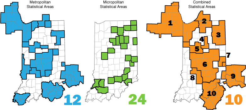
In this example, Indiana has 12 Metropolitan Areas and 24 Micropolitan Areas, which are part of 10 Metropolitan Regions known as Combined Statistical Areas. Out of these CSAs, 7 are within Indiana and 3 extend into neighboring states but include Indiana towns and cities.
The CBSA geographies are formed by combining all of the Metro and Micro areas into a single catalog, but they are all still distinct and mutually exclusive. The CSA geographies are formed by combining multiple Metro and Micro units into aggregated regional units.
939 Core-Based Statistical Areas =
    384 Metropolitan statistical areas +
    547 micropolitan statistical areas

175 Total Combined Statistical Areas:
    808 Metro + Micro Areas joined together to form CSAs
    123 Metro + Micro Areas are not part of any CSA
Before settling on a default geographic unit for your study, it’s a good idea to delve into the definitions a bit. This is important because the choice of geographies ultimately determines how data are aggregated, and what insights you can gain or might miss because of the chosen geographic scale.
HARMONIZED CENSUS FILES
Census geographies change frequently to reflect changes to the underlying administrative units, such as zip codes and voting districts. The formal census boundaries, represented by blocks and tracts, undergo revisions every decade to maintain a balanced population distribution.
Blocks aim to contain between 600 and 3,000 individuals (ideally 1,800), while tracts contain between 1,200 and 8,000 people (ideally 4,000). To achieve this balance, blocks and tracts can have their boundaries redrawn, be divided into multiple units if population density increases, or be combined if the population declines.
Because of these changes, geo-IDs do not consistently measure the same populations over time. This inconsistency can be resolved by standardizing the data to a specific period using an apportionment process. This process uses changes in geographic units over time to update earlier census estimates, making them consistent with the current geographic framework.
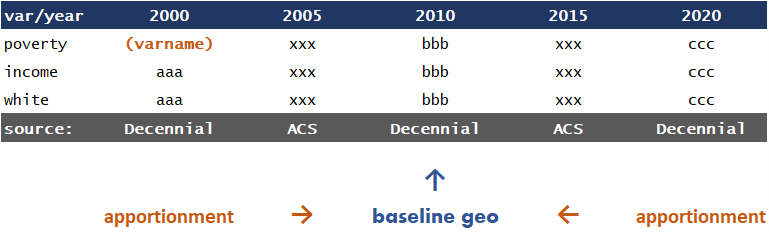
For example, if a tract is split into two new tracts, previous census datasets should also represent this change by dividing the original tract into two parts. These splits are made by approximating the size or density of the new tracts in relation to the original one.
Harmonization can work in both directions, translating past data to fit current geographies or vice versa. Harmonized datasets require a reference period, which is the geography used as the reference for all years of data.
Another challenge in creating a panel of census variables is that different census processes may measure a single variable at different periods. For example, a variable can be measured differently in the American Community Survey and the Decennial Census.
Locating all versions of a single variable can be challenging since table names and variable names change each year. Moreover, some variables are only available for small geographies like blocks during census decades. The American Community Survey doesn’t generate enough observations to accurately estimate the variable at very fine geographical scales.
To address these issues, we have selected a set of the most commonly used census variables and created data files harmonized to the 2010 census geography, serving as the most common reference point across most data sources. These harmonized files are available at the block and tract levels. Most measures can be “aggregated up” to your desired geography level using the geocrosswalk files.
Default Census Variables
A small set of census variables described in this data dictionary have been harmonized to 2010 geographies and inflation-adjusted to the year 2021.
They are available for TRACT, COUNTY, and MSA levels of aggregation:
URL <- "https://raw.githubusercontent.com/UI-Research/nccs-geo/main/get_census_data.R"
source( URL )

df  <- get_census_data( geo="msa" )      # 918 metro areas, all years
df  <- get_census_data( geo="county" )   # 3,142 counties, all years
df  <- get_census_data( geo="tract" )    # 72,597 tracts, all years

# default format is 'long' (stacked years)
df  <- get_census_data( geo="msa", years=2010:2019 )

# return data in a wide format:
dfw <- get_census_data( geo="msa", years=c(1990,2000,2010), format="wide" )

# available years
c(  1990, 2000, 2007, 2008, 2009, 2010, 2011, 2012,
    2013, 2014, 2015, 2016, 2017, 2018, 2019  )
Or you can download files directly via the DATA DOWNLOAD page.
Data Dictionary
| variable_name | variable_description |
|---|---|
| year | Year of data |
| geoid | Geographic identifier |
| total_population | Total population |
| housing_units | Number of housing units |
| occupied | Number of occupied housing units |
| vacant | Number of vacant housing units |
| renter_occ | Number of renter occupied units |
| white_perc | Percent of population that is white |
| black_perc | Percent of population that is black |
| asian_perc | Percent of population that is asian |
| hawaiian_perc | Percent of population that is hawaiian |
| american_alaskan_perc | Percent of population that is american indican or alaskan native |
| two_or_more_perc | Percent of population with two or more races |
| other_perc | Percent of population with race classified as other |
| rural_perc | Percent of population living in rural areas |
| bachelors_perc | Percent of population 25 and over that have a bachelors degree or more |
| hispanic_perc | Percent of population that is hispanic |
| poverty_perc | Percent of population for whom poverty status is determined living in poverty |
| unemployment | Percent of population aged 16 or over and in labor force that are unemployed |
| turnover_perc | Percent of population that moved in the past year |
| med_family_income_adj | Median family income, inflation adjusted to 2021 dollars |
| med_gross_rent_adj | Median gross rent, inflation adjusted to 2021 dollars |
| med_household_income_adj | Median household income, inflation adjusted to 2021 dollars |
| median_value_adj | Median housing value, inflation adjusted to 2021 dollars |
Nonprofit Data Files
In the NCCS system, all nonprofit data that include address information describing the locations of nonprofits or services are geocoded. This process generates latitude and longitude coordinates for these organizations or activities. The resulting geographic coordinate is matched to census blocks using a SPATIAL JOIN.
If you are working with custom data that contains address fields but no latitude and longitude spatial coordinates you might find this GEO PREP TUTORIAL helpful.
Some of the NCCS files contain a block GEOID and a tract GEOID, which include census block FIPS and tract FIPS. You can use these fields to append whichever geographic level you want using the BLOCKX.csv and TRACTX.csv files.
To access the harmonized census panels, refer to the data catalog provided in the “Download” link above.
Feedback
This project is in active development. If you have questions or feedback please open a GitHub Issue in the geocrosswalk repo.
527 Political Action Committees
Electronic filings made by 527 organizations.
Business Master File (BMF)
All active organizations that have been granted nonprofit status by the IRS.